Basics on scRL

Scanpy is not necessary for scRL’s core functions, we utilize it for data loading and parts of visualization, which can be performed mainly by matplotlib and seaborn.

[2]:

import scRL
import scanpy as sc
sc.set_figure_params(figsize=(5,5),frameon=False,fontsize=14)

import matplotlib.pyplot as plt
import seaborn as sns

import pandas as pd
import numpy as np

import warnings
warnings.filterwarnings('ignore')

Preprocessing of the data

[3]:

adata = sc.datasets.paul15()
sc.pp.normalize_total(adata,target_sum=1e4)
sc.pp.log1p(adata)
sc.pp.scale(adata,max_value=10)
sc.pp.pca(adata,n_comps=50)
sc.tl.tsne(adata,perplexity=50)
sc.pp.neighbors(adata)
sc.tl.leiden(adata)

2025-06-01 22:14:11.835777: I tensorflow/core/util/port.cc:113] oneDNN custom operations are on. You may see slightly different numerical results due to floating-point round-off errors from different computation orders. To turn them off, set the environment variable `TF_ENABLE_ONEDNN_OPTS=0`.
2025-06-01 22:14:11.965496: E external/local_xla/xla/stream_executor/cuda/cuda_fft.cc:479] Unable to register cuFFT factory: Attempting to register factory for plugin cuFFT when one has already been registered
2025-06-01 22:14:12.022824: E external/local_xla/xla/stream_executor/cuda/cuda_dnn.cc:10575] Unable to register cuDNN factory: Attempting to register factory for plugin cuDNN when one has already been registered
2025-06-01 22:14:12.023276: E external/local_xla/xla/stream_executor/cuda/cuda_blas.cc:1442] Unable to register cuBLAS factory: Attempting to register factory for plugin cuBLAS when one has already been registered
2025-06-01 22:14:12.124918: I tensorflow/core/platform/cpu_feature_guard.cc:210] This TensorFlow binary is optimized to use available CPU instructions in performance-critical operations.
To enable the following instructions: AVX2 AVX_VNNI FMA, in other operations, rebuild TensorFlow with the appropriate compiler flags.
2025-06-01 22:14:12.942933: W tensorflow/compiler/tf2tensorrt/utils/py_utils.cc:38] TF-TRT Warning: Could not find TensorRT

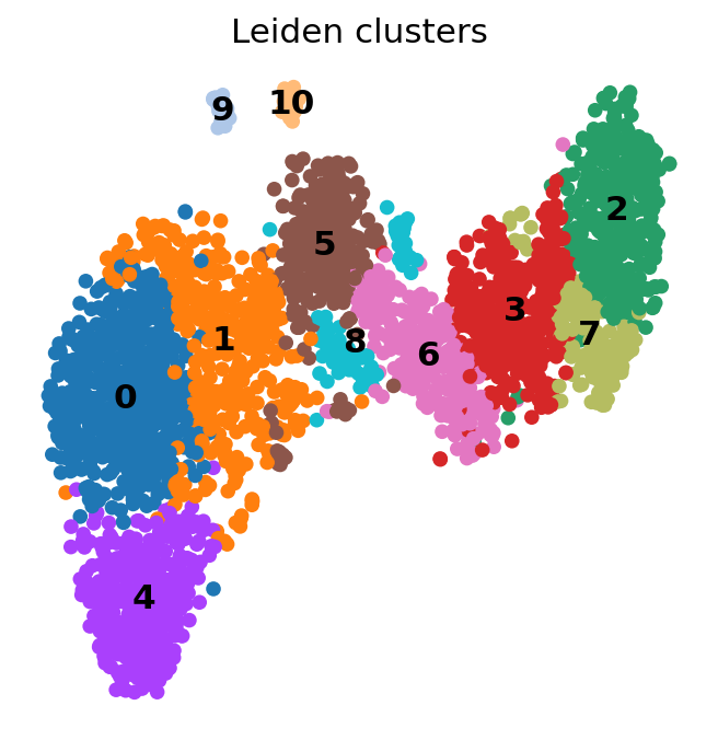
Here we choose the t-SNE output of scanpy as scRL’s 2-D embedding and using the leiden clusters as cell annotations.

[4]:

sc.pl.tsne(adata, color='leiden',legend_loc='on data',s=150, title='Leiden clusters')

../_images/notebook_Basics_on_scRL_6_0.png

scRL’s grid embedding and pseudotime alignment functions

Getting the necessary information for the initialization of scRL.

[5]:

X = adata.obsm['X_tsne']

clusters = adata.obs['leiden']

clusters_colors = adata.uns['leiden_colors']

Generating a grid embedding for the original t-SNE.

[6]:

gres = scRL.grids_from_embedding(X)

Boundary generating: 100%|███████████████████| 196/196 [00:01<00:00, 100.95it/s]
Mask testing: 100%|███████████████████████████████| 8/8 [00:00<00:00, 45.87it/s]
Adjacent generating: 100%|████████████████| 1235/1235 [00:00<00:00, 5594.46it/s]
Boundary pruning: 100%|████████████████████| 271/271 [00:00<00:00, 14716.28it/s]
Adjacent generating: 100%|████████████████| 1300/1300 [00:00<00:00, 5822.19it/s]

Time used for mapping grids: 6.13 seconds

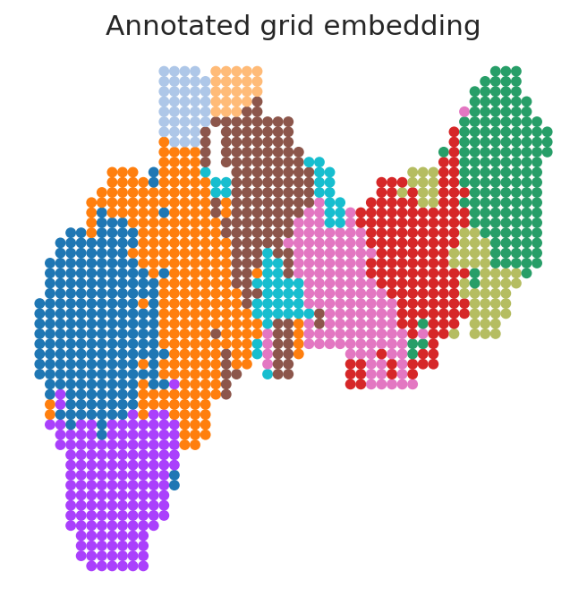
Projecting the annotation information onto the grid embedding space.

[7]:

scRL.project_cluster(gres, clusters, clusters_colors)

Time used for projecting annotation : 0.96 seconds

Select cluster 4 as starting points and aligning pseudotime.

[8]:

scRL.align_pseudotime(gres, '4')

scRL.project_back(gres,'pseudotime')

Time used for aligning pseudo-time : 0.35 seconds

Plotting the grids embedding.

[9]:

g = gres.grids['grids'][gres.grids['mapped_grids']]

[10]:

b = gres.grids['grids'][gres.grids['mapped_boundary']]

[11]:

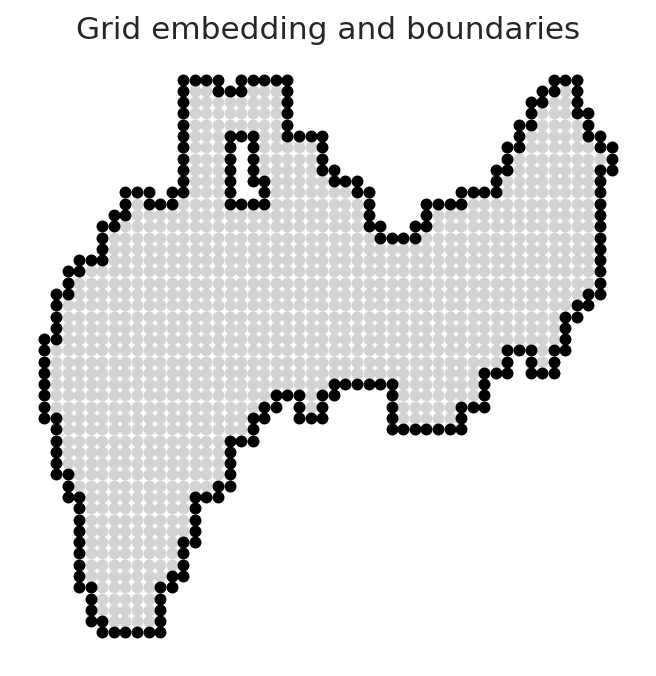
with sns.axes_style('white'):
    plt.scatter(g[:,0], g[:,1], marker='.',s=75,c='lightgrey')
    plt.scatter(b[:,0], b[:,1], marker='.',s=75,c='k')
    ax = plt.gca()
    ax.set_frame_on(False)
    ax.tick_params(labelleft=False, labelbottom=False)
    ax.set_title('Grid embedding and boundaries')

../_images/notebook_Basics_on_scRL_19_0.png

[12]:

with sns.axes_style('white'):
    plt.scatter(g[:,0], g[:,1], marker='.',s=75,c=gres.grids['mapped_grids_colors'])
    ax = plt.gca()
    ax.set_frame_on(False)
    ax.tick_params(labelleft=False, labelbottom=False)
    ax.set_title('Annotated grid embedding')

../_images/notebook_Basics_on_scRL_20_0.png

[13]:

adata.obs['scRL_time'] = gres.embedding['pseudotime']

[14]:

sc.pl.tsne(adata, color='scRL_time', frameon=False,s=150,cmap='viridis',colorbar_loc=None,legend_loc=None,show=False)

[14]:

<Axes: title={'center': 'scRL_time'}, xlabel='tSNE1', ylabel='tSNE2'>

../_images/notebook_Basics_on_scRL_22_1.png

[15]:

sc.pl.tsne(adata, color='Mpo', frameon=False,s=150,cmap='rocket',colorbar_loc=None,legend_loc=None,show=False)

[15]:

<Axes: title={'center': 'Mpo'}, xlabel='tSNE1', ylabel='tSNE2'>

../_images/notebook_Basics_on_scRL_23_1.png

[16]:

exp = pd.DataFrame(adata[:,['Mpo','Klf1']].X,columns=['Mpo','Klf1'])

[18]:

scRL.project(gres, exp)

[20]:

gres.grids.keys()

[20]:

dict_keys(['n', 'grids', 'masked_grids', 'mapped_grids', 'mapped_adj', 'mapped_boundary', 'mapped_travel', 'mapped_grids_clusters', 'mapped_grids_colors', 'pseudotime', 'proj'])

[21]:

with sns.axes_style('white'):
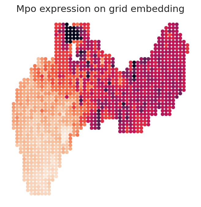
    plt.scatter(g[:,0], g[:,1], marker='.',s=75, c=gres.grids['proj']['Mpo'])
    ax = plt.gca()
    ax.set_frame_on(False)
    ax.tick_params(labelleft=False, labelbottom=False)
    ax.set_title('Mpo expression on grid embedding')

../_images/notebook_Basics_on_scRL_27_0.png

scRL’s reward functions

Decision reward mode for lineage.

[22]:

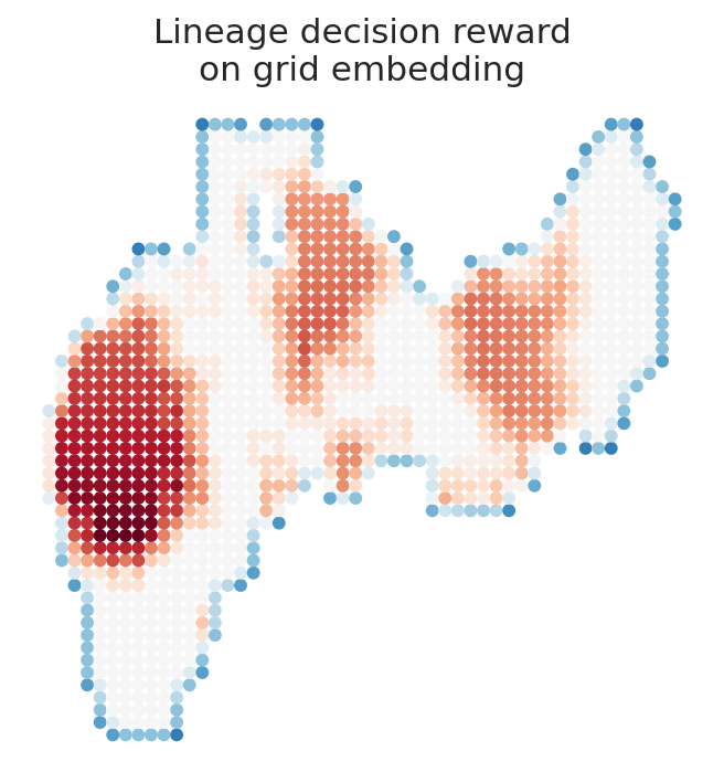
scRL.d_rewards(gres, starts='4', ends=['0','3','5'], mode='Decision')

Reward generating: 100%|██████████████████| 1300/1300 [00:00<00:00, 3508.80it/s]

Time used for generating rewards : 0.39 seconds

[23]:

import matplotlib as mpl

Reward generated

[26]:

with sns.axes_style('white'):
    plt.scatter(g[:,0], g[:,1], marker='.',s=75, c=gres.qlearning['d_Decision_rewards'].sum(axis=1), cmap='RdBu_r', norm=mpl.colors.CenteredNorm())
    ax = plt.gca()
    ax.set_frame_on(False)
    ax.tick_params(labelleft=False, labelbottom=False)
    ax.set_title('Lineage decision reward\non grid embedding')

../_images/notebook_Basics_on_scRL_33_0.png

Training functions

Fetching the PC space for constructing environment and feed the network

[27]:

X_pca = adata.obsm['X_pca']

[30]:

t_mye = scRL.trainer('ActorCritic', gres, reward_type='d', starts_prob=False, X_latent=X_pca, num_episodes=5e3)

r_l, v_l = t_mye.train()

Iteration1: 100%|█████████████| 500/500 [00:06<00:00, 74.88it/s, E=500, R=15.17]
Iteration2: 100%|████████████| 500/500 [00:08<00:00, 59.26it/s, E=1000, R=18.39]
Iteration3: 100%|████████████| 500/500 [00:08<00:00, 62.12it/s, E=1500, R=17.84]
Iteration4: 100%|████████████| 500/500 [00:07<00:00, 63.87it/s, E=2000, R=17.18]
Iteration5: 100%|████████████| 500/500 [00:08<00:00, 60.70it/s, E=2500, R=18.55]
Iteration6: 100%|████████████| 500/500 [00:08<00:00, 62.37it/s, E=3000, R=19.19]
Iteration7: 100%|████████████| 500/500 [00:08<00:00, 59.04it/s, E=3500, R=18.03]
Iteration8: 100%|████████████| 500/500 [00:08<00:00, 61.25it/s, E=4000, R=19.24]
Iteration9: 100%|████████████| 500/500 [00:08<00:00, 58.65it/s, E=4500, R=19.73]
Iteration10: 100%|███████████| 500/500 [00:08<00:00, 62.41it/s, E=5000, R=18.40]

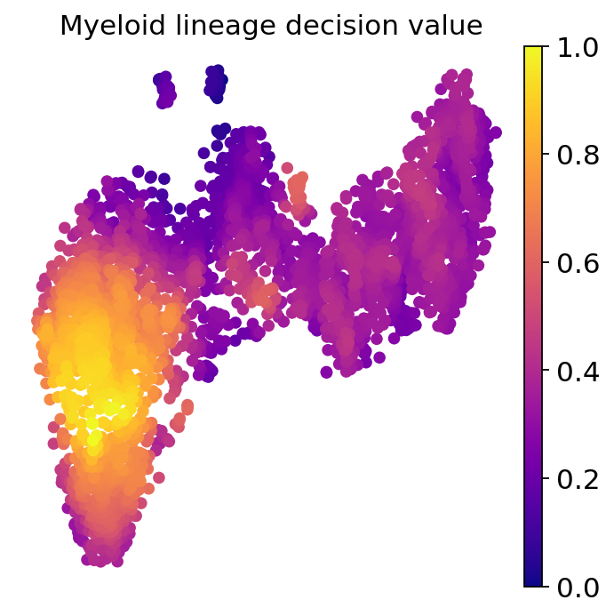
Get the fate decision state value of myeloid lineage

[31]:

scRL.get_state_value(gres, t_mye, 'Mye')

[32]:

scRL.project_back(gres, 'Mye')

[33]:

adata.obs['Mye'] = gres.embedding['Mye']

[34]:

sc.pl.tsne(adata, color='Mye',s=150, cmap='plasma', title=' Myeloid lineage decision value')

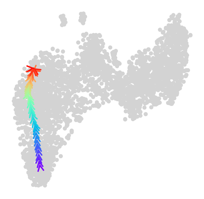
../_images/notebook_Basics_on_scRL_42_0.png

Get the trajectory

[35]:

scRL.get_traj_df(gres, t_mye, key='Mye')

[36]:

scRL.traj_results(gres, [], 'Mye')

../_images/notebook_Basics_on_scRL_45_0.png

[ ]: